
Regularization in Convolutional Neural Networks with PyTorch
How Dropout, Batch Normalization, and Data Augmentation improve model performance in real-world tasks

The Overfitting Trap: Why Your Genius Model Fails the Final Exam
Ever trained a model that scored 99% accuracy on your training data? You felt like a proud parent. But then, you unleashed it on new, unseen data, and it bombed. Hard. What happened? Your model didn’t learn; it memorized.
This is overfitting, the silent killer of machine learning projects. It’s the digital equivalent of a student who crams for a test by memorizing the exact questions and answers from the study guide. They can ace that specific guide, but give them a slightly different question on the same topic, and they freeze. To know more about overfitting and underfitting, check out our blog here
In this guide, we’re going to stop cramming. We’ll become wise teachers, equipping our CNN with powerful techniques like Data Augmentation, Dropout, and Batch Normalization. We’ll turn our model from a mere memorizer into a true master that understands the subject matter, ready for any exam you throw at it.
The Problem with Perfection
In our last article, we built a CNN that did a fantastic job on FashionMNIST. But it learned from a “perfect” world; clean, centered, 28x28 pixel images. The real world is messy. A t-shirt in a photo might be slightly rotated, poorly lit, or a different color. An overfit model is like a hyper-specialized athlete, think of a basketball player who only practices free throws from one exact spot on the court. They might be flawless from that one spot, but move them a foot to the left, and their performance collapses. They learned the position, not the principle of shooting.
Our goal is to build a model that’s more like a seasoned NBA All-Star, someone who can sink a shot from anywhere, under pressure, with defenders in their face. It needs to be resilient, adaptable, and focused on the fundamental patterns; the idea of a t-shirt, not just one specific pixel arrangement of it.
How do we do that? By intentionally making its training a little harder, a little more chaotic. It’s time to introduce some “desirable difficulties.”

Regularization is like Rock Lee training with his ankle weights on, it makes the process harder, but when the weights come off, he’s far stronger and faster than before.
Your Toolkit for Robust Models
Let’s meet the three heroes who will save our model from itself. Think of them as the Gandalf, Dumbledore, and Obi-Wan Kenobi of deep learning wise guides who help our hero (the model) reach its true potential.
1. Data Augmentation
Intuition: If you want your model to recognize a sneaker, you should show it sneakers from every conceivable angle, in different lighting, maybe even partially scuffed up. But what if you only have a limited dataset? You fake it! Data Augmentation creates new, slightly modified training samples from the ones you already have. It’s like a sparring partner in a video game that keeps changing its attack patterns, forcing you to get genuinely good instead of just memorizing a sequence.
We can flip images horizontally (a left shoe is still a shoe), rotate them slightly, or tweak their brightness. This teaches our model the concept of invariance, the core features of an “Ankle boot” are the same even if the photo is tilted by 10 degrees.
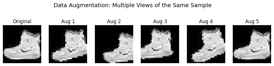
The same boot, seen in slightly different ways. To a model, these are brand new learning opportunities.
2. Dropout
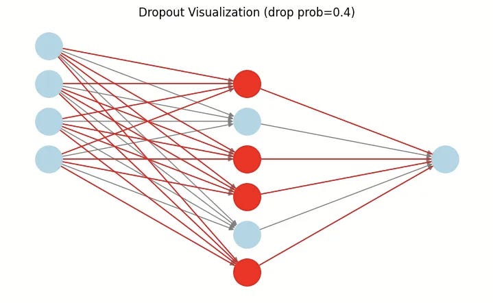
Intuition: Imagine a star player on a basketball team who scores all the points. The team becomes lazy and overly reliant on them. If that star player has an off night, the whole team collapses. This is what happens in a neural network when a few neurons become too dominant.
Dropout is the coach that randomly benches players during practice. On each training iteration, Dropout temporarily and randomly sets some neuron activations to zero. It’s just mind-blowing how simple yet effective this is! The remaining neurons are forced to step up and learn to carry the load. They can’t rely on “that one neuron” to detect the heel of a shoe; they have to learn the feature themselves.
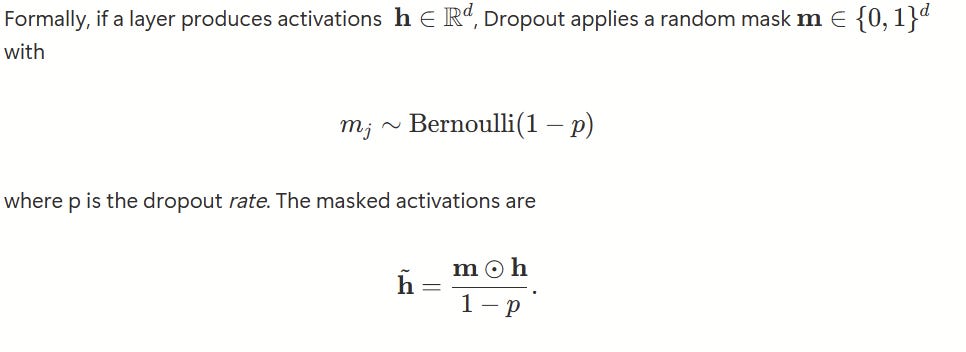
The scaling by 1−p keeps the expected activation magnitude unchanged. At inference time, Dropout is disabled, which is equivalent to averaging predictions over an ensemble of exponentially many thinned subnetworks.
This builds redundancy and forces the network to learn more robust, distributed representations. As the legendary coach Phil Jackson put it, you want to “substitute ‘me’ for ‘we’.” Dropout makes your network a true team.
3. Batch Normalization
Intuition: This one’s a bit more technical, but the analogy is simple. Imagine an orchestra where every musician starts playing without tuning their instruments. The result is chaos. Before a performance, each section tunes to a standard pitch, ensuring they all work together harmoniously.
Batch Normalization (BatchNorm) does this inside your network. As data passes through the layers, the distribution of the outputs (activations) can shift wildly, a problem called “internal covariate shift.” One layer might start outputting values from -1000 to 1000, while the next expects inputs around 0 to 1. It’s a mess! BatchNorm rescales the output of a layer to have a consistent mean (around 0) and standard deviation (around 1) for each mini-batch.
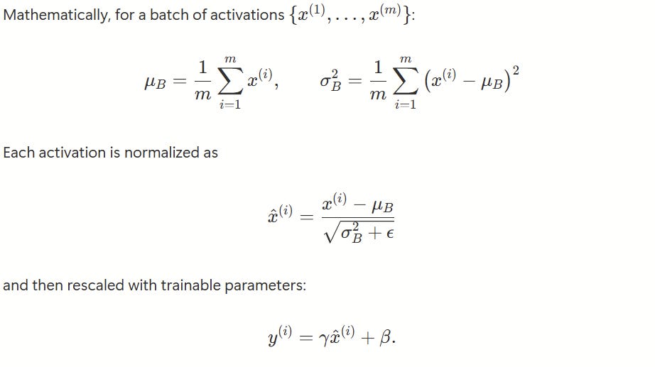
Here, γ and β (shift) restore representational power, and ϵ ensures numerical stability. This keeps the distribution of activations well-behaved across layers and batches.
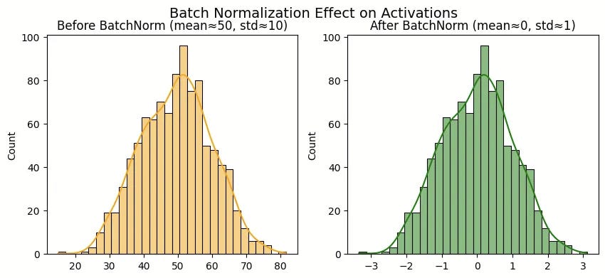
This stabilizes and dramatically speeds up training. It’s like making sure every player in a relay race gets the baton in a predictable, easy-to-handle way, instead of having to catch wild, unpredictable throws.
Let’s Get Our Hands Dirty with PyTorch
Now that we understand the theory, let’s see these techniques in action. We’re going to level up from FashionMNIST to CIFAR-10, a much tougher dataset with 32×32 color images of 10 different object categories: airplanes, automobiles, birds, cats, deer, dogs, frogs, horses, ships, and trucks.
We’re building a deep, VGG-inspired architecture with all three regularization techniques working together.
Step 1: Import the Libraries
First, let’s gather our tools. We’ll need PyTorch for the heavy lifting, torchvision for data handling, and our trusty progress bars to watch the magic happen.
import torch
import torch.nn as nn
import torch.nn.functional as F
import torch.optim as optim
from torch.optim.lr_scheduler import StepLR
from torchvision import datasets, transforms
from torch.utils.data import DataLoader
import matplotlib.pyplot as plt
import numpy as np
from tqdm.auto import tqdm  # For progress bars
Step 2: Data Augmentation
Here’s where we make training deliberately harder. For the training set, we’re going to throw the kitchen sink at our images:
RandomCrop with padding: Shift the image around so the model can’t rely on objects being perfectly centered
RandomHorizontalFlip: A car facing left is still a car
ColorJitter: Mess with brightness, contrast, saturation, and hue so the model learns color-invariant features
But notice: we only augment the training data. The test set uses just normalization. Why? Because we want to evaluate how well our model handles clean, real-world images after being trained in controlled chaos.
data_path = ‘./data’

# Strong augmentation for training—make it HARD
train_transforms = transforms.Compose([
    transforms.RandomCrop(32, padding=4),
    transforms.RandomHorizontalFlip(p=0.5),
    transforms.ColorJitter(brightness=0.2, contrast=0.2,
                          saturation=0.2, hue=0.1),
    transforms.ToTensor(),
    transforms.Normalize((0.4914, 0.4822, 0.4465),
                        (0.2023, 0.1994, 0.2010))
])

# Test data stays clean—only normalization
test_transforms = transforms.Compose([
    transforms.ToTensor(),
    transforms.Normalize((0.4914, 0.4822, 0.4465),
                        (0.2023, 0.1994, 0.2010))
])

# Load the datasets
train_data = datasets.CIFAR10(root=data_path, train=True,
                             download=True, transform=train_transforms)
test_data = datasets.CIFAR10(root=data_path, train=False,
                            download=True, transform=test_transforms)

BATCH_SIZE = 128
train_loader = DataLoader(train_data, batch_size=BATCH_SIZE, shuffle=True)
test_loader = DataLoader(test_data, batch_size=BATCH_SIZE, shuffle=False)

classes = train_data.classes
print(f”Classes: {classes}”)
print(f”Training data batches: {len(train_loader)}”)
print(f”Test data batches: {len(test_loader)}”)
Output:
Classes: [’airplane’, ‘automobile’, ‘bird’, ‘cat’, ‘deer’,
          ‘dog’, ‘frog’, ‘horse’, ‘ship’, ‘truck’]
Training data batches: 391
Test data batches: 79
Step 3: The Model Architecture
This is where BatchNorm and Dropout join the party. Our model is inspired by VGGNet, one of the classic deep architectures. We’re building three convolutional blocks, each going deeper:
Block 1: 3 → 64 channels
Block 2: 64 → 128 channels
Block 3: 128 → 256 channels
Each block follows a pattern: Conv → BatchNorm → ReLU → Conv → BatchNorm → ReLU → MaxPool. This creates a hierarchy of features where early layers detect edges and textures, middle layers detect parts (wheels, wings), and deep layers detect whole objects.
Then in the classifier, we add Dropout(0.5) before the final layer. This is our insurance policy against overfitting.
class AdvancedCNN(nn.Module):
    def __init__(self):
        super().__init__()

        # Convolutional Block 1: Learn basic features
        self.conv_block1 = nn.Sequential(
            nn.Conv2d(3, 64, kernel_size=3, padding=1),
            nn.BatchNorm2d(64),  # Normalize activations
            nn.ReLU(),
            nn.Conv2d(64, 64, kernel_size=3, padding=1),
            nn.BatchNorm2d(64),
            nn.ReLU(),
            nn.MaxPool2d(2, 2)  # 32x32 → 16x16
        )

        # Convolutional Block 2: Learn mid-level features
        self.conv_block2 = nn.Sequential(
            nn.Conv2d(64, 128, kernel_size=3, padding=1),
            nn.BatchNorm2d(128),
            nn.ReLU(),
            nn.Conv2d(128, 128, kernel_size=3, padding=1),
            nn.BatchNorm2d(128),
            nn.ReLU(),
            nn.MaxPool2d(2, 2)  # 16x16 → 8x8
        )

        # Convolutional Block 3: Learn high-level features
        self.conv_block3 = nn.Sequential(
            nn.Conv2d(128, 256, kernel_size=3, padding=1),
            nn.BatchNorm2d(256),
            nn.ReLU(),
            nn.Conv2d(256, 256, kernel_size=3, padding=1),
            nn.BatchNorm2d(256),
            nn.ReLU(),
            nn.MaxPool2d(2, 2)  # 8x8 → 4x4
        )

        # Classifier: Make the final decision
        self.classifier = nn.Sequential(
            nn.Flatten(),
            nn.Linear(256 * 4 * 4, 512),
            nn.ReLU(),
            nn.Dropout(0.5),  # Dropout for regularization!
            nn.Linear(512, 10)
        )

    def forward(self, x):
        x = self.conv_block1(x)
        x = self.conv_block2(x)
        x = self.conv_block3(x)
        x = self.classifier(x)
        return x
Step 4: Training Setup
We’re using the Adam optimizer (a smart, adaptive version of gradient descent) and CrossEntropyLoss (perfect for multi-class classification). But here’s a powerful technique: a Learning Rate Scheduler.
We haven’t spoken about the learning rate scheduler so far. We know that learning rate is our step size when hiking down a mountain to find the lowest valley (optimal weights). Early on, you want big steps to cover ground quickly. But as you get closer to the valley, you need smaller, careful steps to land exactly at the bottom. The scheduler automatically reduces our learning rate by 10× every 10 epochs.
device = torch.device(”cuda” if torch.cuda.is_available() else “cpu”)
print(f”Using device: {device}”)

model = AdvancedCNN().to(device)
criterion = nn.CrossEntropyLoss()
optimizer = optim.Adam(model.parameters(), lr=0.001)

# Scheduler: Reduce LR by 10× every 10 epochs
scheduler = StepLR(optimizer, step_size=10, gamma=0.1)
Step 5: The Training Loop
Here’s where all our techniques come together. For 25 epochs, we:
Train: Feed batches through the model, calculate loss, backpropagate, update weights
Evaluate: Check performance on the untouched test set
Step the scheduler: Adjust the learning rate
Watch what happens to the accuracy over time. This is where the magic becomes visible.
EPOCHS = 25
history = {’train_loss’: [], ‘test_accuracy’: []}

for epoch in range(EPOCHS):
    # --- Training Phase ---
    model.train()  # Enable Dropout and BatchNorm training mode
    running_loss = 0.0
    progress_bar = tqdm(train_loader, desc=f”Epoch {epoch+1}/{EPOCHS}”)

    for images, labels in progress_bar:
        images, labels = images.to(device), labels.to(device)

        optimizer.zero_grad()
        outputs = model(images)
        loss = criterion(outputs, labels)
        loss.backward()
        optimizer.step()

        running_loss += loss.item()
        progress_bar.set_postfix({’loss’: running_loss / len(progress_bar)})

    train_loss = running_loss / len(train_loader)
    history[’train_loss’].append(train_loss)

    # --- Evaluation Phase ---
    model.eval()  # Disable Dropout, use BatchNorm running stats
    correct, total = 0, 0

    with torch.no_grad():
        for images, labels in test_loader:
            images, labels = images.to(device), labels.to(device)
            outputs = model(images)
            _, predicted = torch.max(outputs.data, 1)
            total += labels.size(0)
            correct += (predicted == labels).sum().item()

    test_accuracy = 100 * correct / total
    history[’test_accuracy’].append(test_accuracy)

    scheduler.step()  # Update learning rate

    print(f”Epoch {epoch+1}/{EPOCHS} -> Train Loss: {train_loss:.4f}, “
          f”Test Accuracy: {test_accuracy:.2f}%, “
          f”LR: {scheduler.get_last_lr()[0]:.5f}”)
The Results
Let’s look at what happened epoch by epoch:
Early Epochs (1-10): Rapid Learning
Epoch 1: 50.82% accuracy (barely better than random!)
Epoch 3: 69.18% (the model is seeing the patterns)
Epoch 9: 82.75% (wow, serious progress!)
Mid Epochs (11-20): The Scheduler Kicks In
Epoch 11: 86.57% (learning rate drops, smaller but precise steps)
Epoch 19: 87.91% (steady climbing)
Late Epochs (21-25): Fine-Tuning
Epoch 25: 88.23% (final accuracy!)
Notice how the learning rate dropped from 0.001 → 0.0001 → 0.00001. Each drop gave the model a chance to fine-tune and squeeze out those extra percentage points.
Step 6: Visualizing Success
Numbers are great, but let’s see the learning process visually:
fig, (ax1, ax2) = plt.subplots(1, 2, figsize=(14, 5))

# Plot Training Loss
ax1.plot(history[’train_loss’], label=’Training Loss’, color=’blue’)
ax1.set_title(’Training Loss vs. Epochs’)
ax1.set_xlabel(’Epochs’)
ax1.set_ylabel(’Loss’)
ax1.legend()
ax1.grid(True)

# Plot Test Accuracy
ax2.plot(history[’test_accuracy’], label=’Test Accuracy’, color=’green’)
ax2.set_title(’Test Accuracy vs. Epochs’)
ax2.set_xlabel(’Epochs’)
ax2.set_ylabel(’Accuracy (%)’)
ax2.legend()
ax2.grid(True)

plt.tight_layout()
plt.show()

final_accuracy = history[’test_accuracy’][-1]
print(f”\\nFinal Model Accuracy: {final_accuracy:.2f}%”)
What we see:
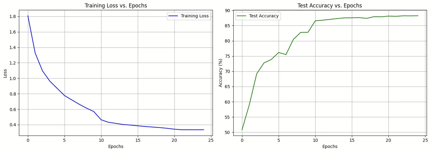
The training loss steadily decreases and smooths out; no wild oscillations, thanks to BatchNorm
Test accuracy climbs rapidly, then plateaus around 88%, this is healthy! It means we’re generalizing, not overfitting
Why This Works
Data Augmentation forced the model to learn invariant features, not memorize specific pixel arrangements
Batch Normalization stabilized training, allowing us to use deeper networks and train faster
Dropout prevented co-adaptation of neurons, creating robust, distributed representations
Learning Rate Scheduling helped the model converge smoothly to an optimal solution
Your Turn: Experiment and Explore
You now have a production-ready CNN template. Here are some ways to push further:
Try different augmentations: Add rotation, translation, or cutout
Adjust dropout rate: Test 0.3, 0.5, or 0.7 and see the impact
Experiment with architecture: Add more layers or try ResNet-style skip connections
Switch datasets: Apply this to CIFAR-100 (100 classes!) or your own image data
Remember: The best models aren’t just smart, they’re resilient. Now go ahead and build models that don’t just memorize, they truly understand! Check out the notebook here to get started.
Key Takeaways and Common Pitfalls
When starting out with regularization, it’s easy to misuse these tools. Here are the most common mistakes and how to avoid them.
1. The “More Is Better” Fallacy
Regularization works like seasoning, effective in moderation, harmful in excess. Setting dropout to extreme values (e.g., 0.9) or overusing BatchNorm will cripple learning instead of improving it.
Guidelines:
Dropout: 0.3–0.5 works well in most cases
Data augmentation: start mild (small rotations, slight color changes)
Avoid BatchNorm just before the final layer
2. Augmenting Test Data
Remember: never, ever augment your test or validation data. Your test set is the final exam, it should represent the real world your model will face. If you augment it, you’re basically giving your student the answers before the test.
3. Forgetting model.eval()
This one’s subtle but deadly. When you call model.eval(), you’re telling PyTorch: “Hey, turn off Dropout and use the running statistics for BatchNorm.” If you forget this during evaluation, your Dropout is still randomly killing neurons, and your accuracy will be artificially low and inconsistent.
model.eval()
with torch.no_grad():
    # evaluation loop
4. Ignoring Training vs. Validation Gap
Track both metrics.
High training, low validation → overfitting
Both low → underfitting
A small gap (2–5%) suggests healthy generalization; a large gap (20%+) signals trouble.
5. Scheduler Misuse
Learning rate schedulers must be stepped explicitly (e.g., scheduler.step()). Defining one without calling it means you won’t benefit from it.
Next Steps
Once you’ve mastered these basics, explore:
ResNets → deeper networks with skip connections
Transfer Learning → fine-tuning pre-trained models to save time and compute. We will cover this in our next article on 6th October 2025.
Advanced Regularization → mixup, cutout, label smoothing
And most importantly, learn to debug systematically. Plot losses, visualize activations, monitor gradients. Improving models is as much about careful diagnosis as it is about clever architectures.
A Final Thought
You know what I love most about deep learning? It’s like chess, you can learn the rules in an hour, but you can spend a lifetime mastering the strategy. The next breakthrough could come from you, sitting in your room, experimenting with ideas that sound crazy until they work.
So go forth. Build. Break things. Fix them. Share your discoveries. And remember what Richard Feynman said: “What I cannot create, I do not understand.”
Resources
PyTorch Docs: The official source is always the best place to learn more about Dropout, BatchNorm2d, and Transforms.
Original Dropout Paper: For the academically curious, read the paper that started it all: Dropout: A Simple Way to Prevent Neural Networks from Overfitting.
Previous Article in this Series: Building and Understanding Convolutional Neural Networks with PyTorch: A Hands-On Guide.