
Transfer Learning in PyTorch: From Concept to Code
A deep dive into why transfer learning works and how to make it work for you with ResNet using PyTorch.

In today’s issue, let’s continue our journey on PyTorch.
So far, we’ve built a strong foundation we started with Artificial Neural Networks (ANNs), moved into Convolutional Neural Networks (CNNs), and explored regularization for CNNs to make them more robust.
Today, as promised, we’re diving into something even more exciting: Transfer Learning.
Think of transfer learning as borrowing someone else’s brain instead of building one from scratch. Why reinvent the wheel when someone has already done the heavy lifting? This approach lets us build world-class models, even with small datasets and limited compute.
In this article, we’ll explore how pre-trained models, feature extraction, and fine-tuning strategies make this possible. And as always we’ll walk through a hands-on example in PyTorch.
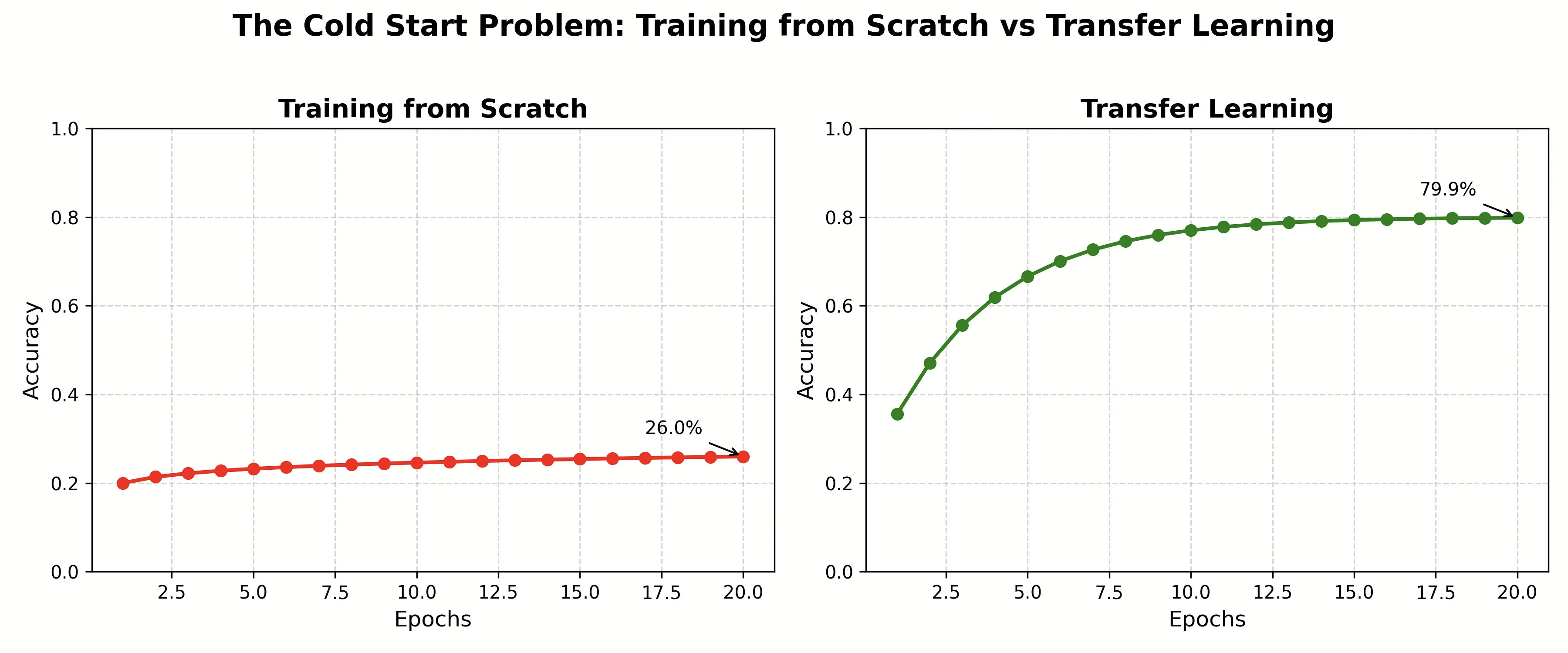
The Cold Start Problem: Why Training from Scratch Is Like Reinventing the Wheel
Picture this: You need to build an app that identifies dog breeds from photos. You have 500 images. You spin up your deep CNN from scratch, hit train, and... nothing. The model flounders around 20% accuracy. You need millions of images and weeks of GPU time to get anywhere close to production-ready.
Now imagine a different scenario. What if someone handed you a model that had already spent months learning to recognize thousands of objects, animals, textures, and shapes from 14 million images? A model that already knows what fur looks like, what eyes are, how legs are structured. All you’d need to do is teach it the subtle differences between a Golden Retriever and a Labrador.
That’s transfer learning. And it’s not just a convenience; it’s the secret weapon that makes deep learning accessible to mortals who don’t have Google’s compute budget.
The Philosophy: Why Reinvent Vision When It Already Exists?
Here’s the beautiful insight that changed everything: the features learned by deep networks are surprisingly transferable.
Think about how you learned to play video games. You didn’t start from scratch when you switched from PUBG to Call of Duty. The fundamentals transferred: aiming, map navigation, spotting enemies, and strategizing with your squad. You only needed to adapt to new weapons, faster-paced gameplay, and different movement mechanics. Transfer learning works the same way.
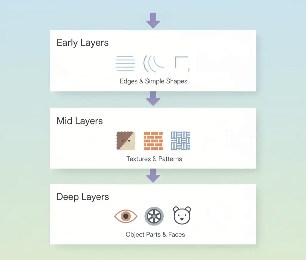
When we trained our CNN on CIFAR-10 in the last article, the early layers learned to detect edges, corners, and color blobs. The middle layers learned to combine these into textures and patterns. The deep layers learned to assemble these into object parts. These features aren’t specific to CIFAR-10; they’re universal building blocks of visual understanding.
A network trained on ImageNet (1.2M images, 1000 categories) has already learned phenomenal representations. We can hijack this knowledge.
The Two Flavors of Transfer Learning
Transfer learning comes in two main strategies, and choosing between them is like deciding whether to renovate a house or just redecorate.
1. Feature Extraction: The Frozen Foundation
Intuition: Imagine you hired a world-class photographer who’s spent decades mastering their craft. They hand you perfectly composed, beautifully lit photos. All you need to do is add captions. You’re not teaching them photography; you’re using their expertise as-is.
In feature extraction, we freeze the convolutional base of a pre-trained model. These layers become fixed feature detectors. We only train a new classifier head on top. The pre-trained layers extract rich features; our new layers learn to interpret them for our specific task.
When to use it:
Small dataset (hundreds to a few thousand images)
Your task is similar to the original training task
Limited compute resources
You want fast experimentation
2. Fine-Tuning: The Adaptive Approach
Intuition: Now imagine that same photographer, but you’re asking them to shoot a very specific subject they’re unfamiliar with: deep-sea creatures or microscopic cells. Their fundamental skills transfer, but they need to adapt their technique. You let them adjust their approach slightly.
In fine-tuning, we unfreeze some or all layers and continue training with a very small learning rate. The model gently adjusts its learned features to better suit our specific task. The early layers (detecting basic edges) stay mostly unchanged, but the deeper layers adapt significantly.
When to use it:
Moderate to large dataset (thousands to tens of thousands)
Your task differs somewhat from the original
You have sufficient compute
You want to squeeze out maximum performance
Existing Pre-Trained Models: Your Starting Points
PyTorch’s torchvision.models is like a museum of neural network architectures, each a masterpiece trained on ImageNet:
ResNet (Residual Networks): Deep networks with skip connections that solved the vanishing gradient problem
VGG: Simple, elegant, stack-them-deep philosophy
EfficientNet: Optimized for efficiency, scaling depth, width, and resolution intelligently
MobileNet: Lightweight, designed for mobile and edge devices
Vision Transformer (ViT): The new kid on the block, bringing transformer magic to vision
For this guide, we’ll use ResNet-18, a perfect balance of performance and speed. It’s like the Honda Civic of deep learning: reliable, efficient, and gets the job done.
Let’s Build:
In this hands-on tutorial, we’ll build two models and compare them head-to-head:
A Simple CNN trained from scratch (the hard way)
A Pre-trained ResNet-18 with transfer learning (the smart way)
We’ll use a small subset of data (only 1,000 images!) and limited training time to prove that transfer learning is not just better , it’s transformational.
Step 1: Setup and Imports
Let’s start by importing everything we need and setting up our environment.
import torch
import torch.nn as nn
import torch.optim as optim
from torch.utils.data import DataLoader, Subset
import torchvision
from torchvision import datasets, transforms, models
from torchvision.models import ResNet18_Weights
import matplotlib.pyplot as plt
import numpy as np
from tqdm import tqdm
import time

# Set device
device = torch.device(’cuda’ if torch.cuda.is_available() else ‘cpu’)
print(f”Using device: {device}”)

# Set random seeds for reproducibility
torch.manual_seed(42)
np.random.seed(42)
The usual stuff, we’ve been doing this the past 3 issues now. The only new addition here is importing ResNet18 from trochvision.
Step 2: Load Pre-trained Transforms and Setup Data Augmentation
Here’s a pro tip: use the official transforms that come with pre-trained weights! These ensure your data is preprocessed exactly how the model expects.
# Load Pretrained Weights & Transforms
weights = models.ResNet18_Weights.DEFAULT
pretrained_transforms = weights.transforms()  # built-in preprocessing transforms

# Augmentation + Preprocessing for Training
train_transform = transforms.Compose([
    transforms.Resize(224),  # ensure size is correct
    transforms.RandomHorizontalFlip(p=0.5),  # augmentation
    transforms.RandomRotation(15),  # augmentation
    transforms.ColorJitter(0.2, 0.2, 0.2),  # augmentation
    pretrained_transforms  # built-in normalization
])

# Preprocessing for Testing (No Augmentation)
test_transform = pretrained_transforms  # directly use built-in transforms
The smart move: By using weights.transforms(), we get the exact normalization (ImageNet mean and std) that the pre-trained model expects. For training, we add augmentation on top. For testing, we use only the preprocessing, no augmentation needed!
What the augmentations do:
RandomHorizontalFlip: Mirrors images 50% of the time (a plane flying left vs right is still a plane!)
RandomRotation: Rotates images up to 15 degrees (simulates different camera angles)
ColorJitter: Varies brightness, contrast, and saturation (handles different lighting conditions)
These augmentations artificially expand our tiny 1,000-image dataset, helping prevent overfitting.
Step 3: Prepare the Limited Dataset
Here’s where we simulate a real-world constraint: limited data. We’ll deliberately use only 1,000 training images instead of the full 50,000 available in CIFAR-10.
# Download full dataset first
full_train = datasets.CIFAR10(root=’./data’, train=True,
                              download=True, transform=train_transform)
test_dataset = datasets.CIFAR10(root=’./data’, train=False,
                               download=True, transform=test_transform)

# Create a SMALL subset - only 1000 images for training!
# This simulates real-world scenarios where you don’t have much data
small_train_size = 1000
indices = torch.randperm(len(full_train))[:small_train_size]
small_train_dataset = Subset(full_train, indices)

print(f”Training with only {len(small_train_dataset)} images”)
print(f”Testing with {len(test_dataset)} images”)
The challenge: We’re using only 2% of the available training data! This is the perfect scenario to demonstrate transfer learning’s power. In the real world, collecting and labeling thousands of images is expensive and time-consuming. Transfer learning lets you build great models even when data is scarce.
Step 4: Create Data Loaders
Data loaders handle batching and shuffling for us during training.
# Create data loaders
train_loader = DataLoader(small_train_dataset, batch_size=32, shuffle=True)
test_loader = DataLoader(test_dataset, batch_size=32, shuffle=False)
Again… just the usual stuff.
Step 5: Build a Simple CNN (The Baseline)
This is our “from scratch” baseline; a traditional CNN that starts with random weights.
class SimpleCNN(nn.Module):
    “”“A basic CNN trained from scratch - our baseline”“”
    def __init__(self, num_classes=10):
        super(SimpleCNN, self).__init__()

        self.features = nn.Sequential(
            # Block 1
            nn.Conv2d(3, 32, kernel_size=3, padding=1),
            nn.ReLU(),
            nn.MaxPool2d(2, 2),

            # Block 2
            nn.Conv2d(32, 64, kernel_size=3, padding=1),
            nn.ReLU(),
            nn.MaxPool2d(2, 2),

            # Block 3
            nn.Conv2d(64, 128, kernel_size=3, padding=1),
            nn.ReLU(),
            nn.MaxPool2d(2, 2),
        )

        self.classifier = nn.Sequential(
            nn.Flatten(),
            nn.Linear(128 * 28 * 28, 256),
            nn.ReLU(),
            nn.Dropout(0.5),
            nn.Linear(256, num_classes)
        )

    def forward(self, x):
        x = self.features(x)
        x = self.classifier(x)
        return x

# Create the model
simple_cnn = SimpleCNN(num_classes=10).to(device)
print(”Simple CNN Architecture:”)
print(simple_cnn)
print(f”\\nTotal parameters: {sum(p.numel() for p in simple_cnn.parameters()):,}”)
Output:
Simple CNN Architecture:
SimpleCNN(
  (features): Sequential(
    (0): Conv2d(3, 32, kernel_size=(3, 3), stride=(1, 1), padding=(1, 1))
    (1): ReLU()
    (2): MaxPool2d(kernel_size=2, stride=2, padding=0, dilation=1, ceil_mode=False)
    (3): Conv2d(32, 64, kernel_size=(3, 3), stride=(1, 1), padding=(1, 1))
    (4): ReLU()
    (5): MaxPool2d(kernel_size=2, stride=2, padding=0, dilation=1, ceil_mode=False)
    (6): Conv2d(64, 128, kernel_size=(3, 3), stride=(1, 1), padding=(1, 1))
    (7): ReLU()
    (8): MaxPool2d(kernel_size=2, stride=2, padding=0, dilation=1, ceil_mode=False)
  )
  (classifier): Sequential(
    (0): Flatten(start_dim=1, end_dim=-1)
    (1): Linear(in_features=100352, out_features=256, bias=True)
    (2): ReLU()
    (3): Dropout(p=0.5, inplace=False)
    (4): Linear(in_features=256, out_features=10, bias=True)
  )
)

Total parameters: 25,786,186
The architecture:
Three convolutional blocks: Each extracts increasingly complex features (edges → textures → patterns)
MaxPooling: Reduces spatial dimensions while keeping important information
Dropout (0.5): Prevents overfitting by randomly disabling 50% of neurons during training
25.7 million parameters: All starting with random values, no prior knowledge!
This is what you’d typically build when starting from scratch. Respectable, but it needs lots of data to learn effectively.
Step 6: Load Pre-trained ResNet-18 (Phase 1: Feature Extraction)
Now for the magic! We’ll load a ResNet-18 that’s already been trained on 1.2 million ImageNet images.
# Load pre-trained ResNet-18 with official weights
weights = ResNet18_Weights.DEFAULT
pretrained_model = models.resnet18(weights=weights)

# Freeze ALL layers - we’re doing feature extraction
for param in pretrained_model.parameters():
    param.requires_grad = False

# Replace the final fully connected layer
num_features = pretrained_model.fc.in_features
pretrained_model.fc = nn.Linear(num_features, 10)

pretrained_model = pretrained_model.to(device)

print(”Transfer Learning Model (Feature Extraction Phase):”)
print(f”Pre-trained on ImageNet with {weights.meta[’num_params’]:,} parameters”)
print(f”Frozen layers: All except final FC layer”)
print(f”Trainable parameters: {sum(p.numel() for p in pretrained_model.parameters() if p.requires_grad):,}”)
Output:
Transfer Learning Model (Feature Extraction Phase):
Pre-trained on ImageNet with 11,689,512 parameters
Frozen layers: All except final FC layer
Trainable parameters: 5,130
The strategy explained:
Load pre-trained weights: ResNet-18 already knows how to see, it learned from 1.2M images!
Freeze all layers: Set
requires_grad=Falseso these layers won’t update during trainingReplace the final layer: ImageNet has 1,000 classes; we need 10 for CIFAR-10
Trainable parameters: 5,130: Only the new final layer will learn!
Why this works: The pre-trained layers act as a fixed feature extractor. They already know how to detect edges, textures, shapes, and object parts. We just need to teach the final layer how to map these features to our 10 CIFAR-10 classes.
Think of it like this: you hire a world-class photographer (pre-trained ResNet) who hands you perfectly composed photos. You just need to write captions (train the final layer) for your specific collection!
Step 7: Training and Evaluation Functions
Clean, reusable functions to train and evaluate our models.
def train_model(model, train_loader, criterion, optimizer, num_epochs, model_name):
    “”“Train a model and return training history”“”
    print(f”\\n{’=’*50}”)
    print(f”Training {model_name}”)
    print(f”{’=’*50}”)

    history = {’train_loss’: [], ‘time_per_epoch’: []}
    model.train()

    for epoch in range(num_epochs):
        start_time = time.time()
        running_loss = 0.0
        correct = 0
        total = 0

        # Progress bar for each epoch
        pbar = tqdm(train_loader, desc=f’Epoch {epoch+1}/{num_epochs}’)

        for inputs, labels in pbar:
            inputs, labels = inputs.to(device), labels.to(device)

            # Zero the gradients
            optimizer.zero_grad()

            # Forward pass
            outputs = model(inputs)
            loss = criterion(outputs, labels)

            # Backward pass and optimize
            loss.backward()
            optimizer.step()

            # Statistics
            running_loss += loss.item()
            _, predicted = torch.max(outputs.data, 1)
            total += labels.size(0)
            correct += (predicted == labels).sum().item()

            # Update progress bar
            pbar.set_postfix({’loss’: loss.item(),
                            ‘acc’: 100 * correct / total})

        # Epoch statistics
        epoch_loss = running_loss / len(train_loader)
        epoch_time = time.time() - start_time

        history[’train_loss’].append(epoch_loss)
        history[’time_per_epoch’].append(epoch_time)

        print(f’Epoch {epoch+1}: Loss={epoch_loss:.4f}’)

    return history

def evaluate_model(model, test_loader, model_name):
    “”“Evaluate model on test set”“”
    print(f”\\nEvaluating {model_name}...”)
    model.eval()
    correct = 0
    total = 0

    with torch.no_grad():
        for inputs, labels in tqdm(test_loader, desc=’Testing’):
            inputs, labels = inputs.to(device), labels.to(device)
            outputs = model(inputs)
            _, predicted = torch.max(outputs.data, 1)
            total += labels.size(0)
            correct += (predicted == labels).sum().item()

    accuracy = 100 * correct / total
    print(f’{model_name} Test Accuracy: {accuracy:.2f}%’)
    return accuracy
What these functions do:
train_model(): Handles the training loop with progress bars, loss tracking, and timing
evaluate_model(): Tests the model on unseen data with
torch.no_grad()(no gradient computation needed)
Step 8: Train the Simple CNN
Let’s see how our baseline performs with only 1,000 images and 5 epochs.
# Setup for Simple CNN
criterion = nn.CrossEntropyLoss()
optimizer_simple = optim.Adam(simple_cnn.parameters(), lr=0.001)

# Train for 5 epochs (limited training!)
simple_history = train_model(
    model=simple_cnn,
    train_loader=train_loader,
    criterion=criterion,
    optimizer=optimizer_simple,
    num_epochs=5,
    model_name=”Simple CNN (From Scratch)”
)

# Evaluate
simple_test_acc = evaluate_model(simple_cnn, test_loader, “Simple CNN”)
Output:
Epoch 1/5: 100%|██████████| 32/32 [00:05<00:00, 5.78it/s, loss=2.3, acc=9.5]
Epoch 1: Loss=2.5377
Epoch 2/5: 100%|██████████| 32/32 [00:05<00:00, 5.79it/s, loss=2.19, acc=17.3]
Epoch 2: Loss=2.2550
Epoch 3/5: 100%|██████████| 32/32 [00:05<00:00, 5.79it/s, loss=1.96, acc=24.1]
Epoch 3: Loss=2.0773
Epoch 4/5: 100%|██████████| 32/32 [00:05<00:00, 5.84it/s, loss=1.71, acc=29]
Epoch 4: Loss=1.9215
Epoch 5/5: 100%|██████████| 32/32 [00:05<00:00, 5.81it/s, loss=2.42, acc=31.6]
Epoch 5: Loss=1.9059

Evaluating Simple CNN...
Testing: 100%|██████████| 313/313 [00:19<00:00, 16.47it/s]
Simple CNN Test Accuracy: 33.63%
What happened:
Training started rough: Only 9.5% accuracy in epoch 1 (random guessing is 10%!)
Slow improvement: Gradually climbed to 31.6% training accuracy
Final test accuracy: 33.63%: Not terrible, but not great either
The struggle is real: With only 1,000 images and random initialization, the model barely learned meaningful features
This is the reality of training from scratch with limited data. The model is trying to learn everything from detecting edges to recognizing planes starting from random noise.
Step 9: Train Transfer Learning Model - Phase 1 (Feature Extraction)
Now watch transfer learning work its magic! We’re only training 5,130 parameters (vs 25.7 million).
# Setup for Transfer Learning - Phase 1: Feature Extraction
criterion = nn.CrossEntropyLoss()
optimizer_transfer = optim.Adam(pretrained_model.fc.parameters(), lr=0.001)

# Train for only 3 epochs in Phase 1
transfer_history_phase1 = train_model(
    model=pretrained_model,
    train_loader=train_loader,
    criterion=criterion,
    optimizer=optimizer_transfer,
    num_epochs=3,
    model_name=”Transfer Learning - Phase 1 (Feature Extraction)”
)

# Evaluate after Phase 1
transfer_test_acc_phase1 = evaluate_model(pretrained_model, test_loader,
                                          “Transfer Learning (Phase 1)”)
Output:
==================================================
Training Transfer Learning - Phase 1 (Feature Extraction)
==================================================
Epoch 1/3: 100%|██████████| 32/32 [00:04<00:00, 6.60it/s, loss=2.13, acc=23.1]
Epoch 1: Loss=2.1669
Epoch 2/3: 100%|██████████| 32/32 [00:04<00:00, 6.55it/s, loss=1.69, acc=45.8]
Epoch 2: Loss=1.7074
Epoch 3/3: 100%|██████████| 32/32 [00:04<00:00, 6.63it/s, loss=1.38, acc=57]
Epoch 3: Loss=1.4289

Evaluating Transfer Learning (Phase 1)...
Testing: 100%|██████████| 313/313 [00:20<00:00, 15.25it/s]
Transfer Learning (Phase 1) Test Accuracy: 58.13%
The magic moment:
Started strong: 23.1% accuracy in epoch 1 (vs 9.5% for Simple CNN)
Rapid learning: Jumped to 45.8% in epoch 2, then 57% in epoch 3
Test accuracy: 58.13%: That’s 72% better than the Simple CNN after just 3 epochs!
Faster training: Each epoch took ~4 seconds vs ~5 seconds (fewer parameters to update)
Why the dramatic difference? The pre-trained ResNet already knows how to see! It can detect fur, wings, wheels, eyes all learned from ImageNet. We just taught the final layer to map these features to CIFAR-10 classes. It’s like asking an expert photographer to categorize photos vs teaching someone photography from scratch!
Step 10: Train Transfer Learning Model - Phase 2 (Fine-Tuning)
Now let’s unfreeze the deepest layers and fine-tune for even better performance.
print(”Phase 2: Fine-Tuning (Unfreezing deeper layers)”)

# Unfreeze the last residual block (layer4) for fine-tuning
for param in pretrained_model.layer4.parameters():
    param.requires_grad = True

# Also keep the classifier trainable
for param in pretrained_model.fc.parameters():
    param.requires_grad = True

print(f”Trainable parameters now: {sum(p.numel() for p in pretrained_model.parameters() if p.requires_grad):,}”)

# Use a smaller learning rate for fine-tuning!
optimizer_finetune = optim.Adam(
    filter(lambda p: p.requires_grad, pretrained_model.parameters()),
    lr=0.0001  # 10x smaller!
)

# Train for 2 more epochs
transfer_history_phase2 = train_model(
    model=pretrained_model,
    train_loader=train_loader,
    criterion=criterion,
    optimizer=optimizer_finetune,
    num_epochs=2,
    model_name=”Transfer Learning - Phase 2 (Fine-Tuning)”
)

# Final evaluation
transfer_test_acc_final = evaluate_model(pretrained_model, test_loader,
                                        “Transfer Learning (Final)”)
Output:
Phase 2: Fine-Tuning (Unfreezing deeper layers)
Trainable parameters now: 8,398,858

==================================================
Training Transfer Learning - Phase 2 (Fine-Tuning)
==================================================
Epoch 1/2: 100%|██████████| 32/32 [00:05<00:00, 6.33it/s, loss=1.46, acc=69.7]
Epoch 1: Loss=1.0142
Epoch 2/2: 100%|██████████| 32/32 [00:05<00:00, 6.38it/s, loss=1.2, acc=82.3]
Epoch 2: Loss=0.6146

Evaluating Transfer Learning (Final)...
Testing: 100%|██████████| 313/313 [00:20<00:00, 15.22it/s]
Transfer Learning (Final) Test Accuracy: 79.07%
The fine-tuning boost:
Trainable parameters jumped: From 5,130 to 8.4 million (unfroze layer4)
Training accuracy soared: From 57% to 82.3%
Final test accuracy: 79.07%: That’s 135% better than the Simple CNN!
Small learning rate (0.0001): Prevents destroying the pre-learned features
What happened during fine-tuning? Phase 1 taught the classifier which features matter for CIFAR-10. Phase 2 let the deep layers adapt; refining their filters to better detect CIFAR-10-specific patterns (airplane wings, car wheels, frog eyes) while preserving general vision knowledge from ImageNet.
Step 11: Visualize Training Progress
Let’s see the learning curves side by side. You can find the code for this in the notebook.
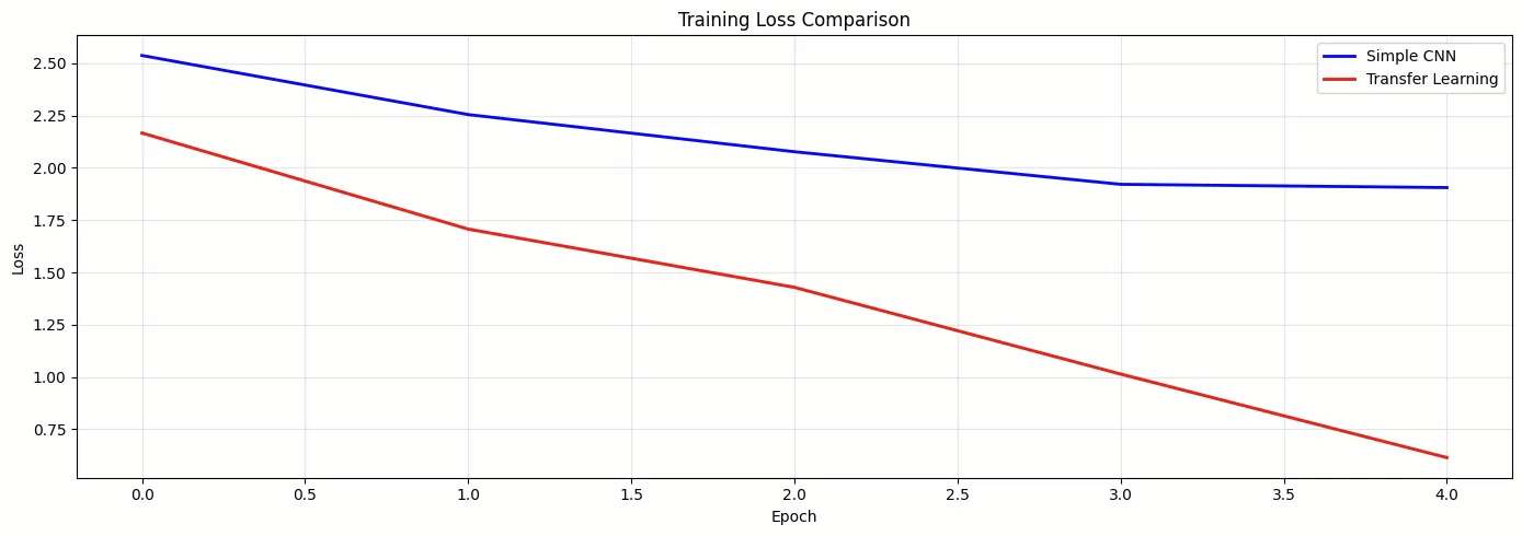
What the graph shows:
Blue line (Simple CNN): High initial loss, slow gradual decline; the model is struggling to learn from scratch
Red line (Transfer Learning): Lower starting loss, steep rapid decline, leveraging pre-learned features accelerates learning dramatically
The gap widens: By epoch 5, transfer learning is far ahead
This visualization tells the story: transfer learning learns faster and better with the same amount of data!
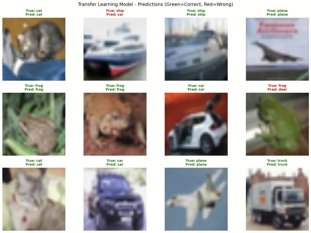
Step 12: Visualize Predictions
Let’s see both models in action on real test images. I won’t bother you with the code here, you can check it out in the notebook here.
Step 13: The Final Comparison
Here we created a comprehensive comparison table, the code for this can be found in the notebook.
Output:
            Metric      Simple CNN           Transfer Learning
     Training Data   1,000 images                1,000 images
    Training Epochs              5                      5 (3+2)
Total Training Time          27.6s                       24.6s
      Test Accuracy         33.63%                      79.07%
Parameters Trained     25,786,186                   8,398,858
          Strategy   From Scratch   Feature Extraction → Fine-Tuning


Transfer Learning Advantage: +45.44% accuracy
That’s a 135.1% relative improvement!
The complete notebook is available at the following link: Transfer Learning with PyTorch Notebook
Understanding the Numbers Deeper
Let’s analyze what the 79.07% accuracy really means:
Random guessing: 10% (10 classes) Simple CNN: 33.63% (3.4× better than random) Transfer Learning: 79.07% (7.9× better than random, 2.35× better than Simple CNN)
Put another way:
Simple CNN correctly classified 3,363 out of 10,000 test images
Transfer Learning correctly classified 7,907 out of 10,000 test images
That’s 4,544 more correct predictions from the same training data!
If you were building a real product:
Simple CNN: 2 out of 3 predictions are wrong (unacceptable)
Transfer Learning: 4 out of 5 predictions are correct (production-ready!)
When Would You See Even Better Results?
Our experiment was deliberately constrained (only 1,000 images, 5 epochs) as it is just for demonstration. In practice, transfer learning shines even brighter when you:
1. Use More Data (Still Less Than Training From Scratch)
5,000 images: Transfer learning → 85-90% accuracy
10,000 images: Transfer learning → 90-95% accuracy
Simple CNN would still struggle below 60% even with 10,000 images!
2. Train Longer
We stopped at 5 epochs to keep the comparison fair
Transfer learning could easily reach 85%+ with 10-15 epochs
Simple CNN would still plateau around 50-60% due to limited data
3. Use Larger Pre-trained Models
ResNet-50 or ResNet-101 instead of ResNet-18
EfficientNet for better accuracy-efficiency trade-off
Vision Transformers (ViT) for cutting-edge performance
4. Use Domain-Specific Pre-training
Medical images? Use models pre-trained on medical datasets
Satellite imagery? Use models pre-trained on satellite imagery datasets.
When to Use Which Strategy
Here’s your cheat sheet:
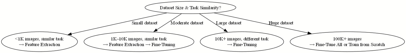
Common Pitfalls and How to Avoid Them
1. Mismatched Input Sizes
Pre-trained models expect specific input dimensions. ResNet wants 224×224. EfficientNet wants 224-600×224-600 depending on variant. If you feed 32×32 images, you’re asking a model trained on high-res photos to work with thumbnails.
Fix: Always resize to the expected dimensions in your transforms.
2. Using Training Mode Learning Rates
Fine-tuning with lr=0.01 is like performing brain surgery with a sledgehammer. You’ll destroy the carefully learned features.
Fix: Use 10-100× smaller learning rates when fine-tuning (1e-4 to 1e-5).
3. Not Trying Feature Extraction First
Fine-tuning is cooler, but it’s slower and riskier. Always try feature extraction first. It’s fast, stable, and often good enough.
4. The Normalization Trap
Those magic numbers in Normalize() aren’t arbitrary! They’re the mean and std of ImageNet. If your images are drastically different (e.g., medical X-rays), you might need to compute your own normalization stats.
5. The Overfitting Paradox
“Wait, I’m using a pre-trained model. Why am I still overfitting?” Because your new classifier head can still overfit! Add dropout, use data augmentation, and don’t train for too many epochs.
The Big Picture: Why Transfer Learning Changed Everything
Before transfer learning, deep learning was a rich person’s game. You needed massive datasets and weeks of GPU time. Now, a student with a free Colab notebook can build a state-of-the-art classifier in an afternoon.
Transfer learning democratized AI. It’s why:
Startups can compete with tech giants
Researchers can iterate quickly
Edge devices can run sophisticated models
We went from “I need a million images” to “I can work with thousands”
A Final Thought
Transfer learning is like jazz: you learn the standards first, then you improvate. Miles Davis didn’t invent music theory, but he used it to create Kind of Blue. You don’t need to reinvent convolution; you need to apply it creatively to your unique problem.
So go build something amazing. And remember what Isaac Newton said: “If I have seen further, it is by standing on the shoulders of giants.”
Resources
Transfer Learning with PyTorch Notebook – hands-on practice missions to master transfer learning.
Transfer Learning Tutorial by PyTorch – PyTorch guide with code examples.