Building and Understanding Artificial Neural Networks: A Comprehensive Guide for Beginners

Learn How Neural Networks Work and Implement Them Using PyTorch

“The mind is not a vessel to be filled, but a fire to be kindled.” – Plutarch

And oh boy, once that fire gets lit with AI, there’s no turning back! Today, we’re going to spark that fire together starting from scratch with Artificial Neural Networks (ANNs) and bringing them to life with PyTorch, one of the coolest tools out there.

Imagine this…

You’re at a crowded cafe, sipping on a caramel latte ☕, when suddenly across the room you spot your best friend waving. Without thinking twice, your brain says, “Hey, that’s them!” How did it know? It didn’t compare every pixel or scan every detail, it recognized a pattern. That’s your brain’s neural network at work!

Now, here’s the crazy part: computers can kinda do this too. They can learn patterns from data, and mimic decision-making all with something called an Artificial Neural Network, or ANN for short. It’s just mind-blowing how science and math together help machines ‘see’ and ‘think’ like us, at least in a very basic way.

What is an Artificial Neural Network? Let’s break it down

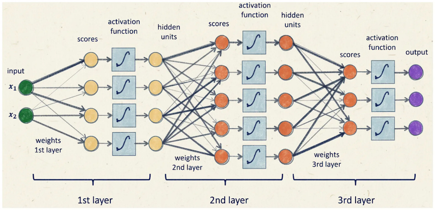
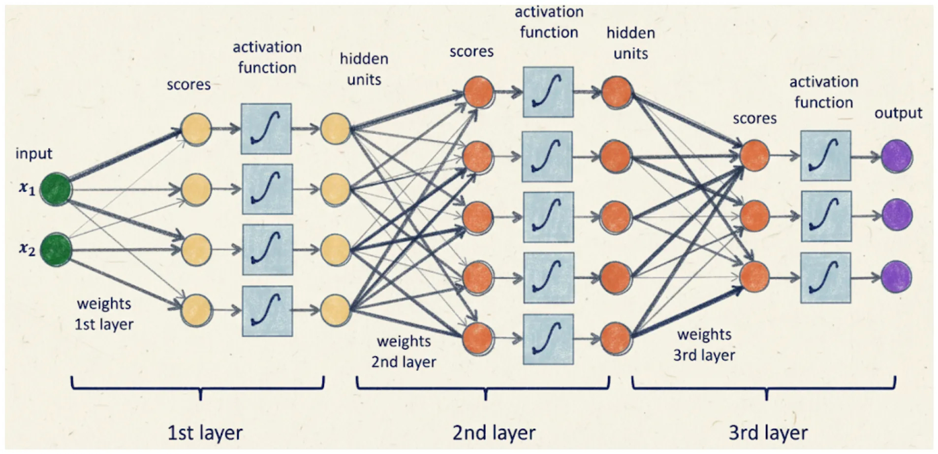
At its core, an ANN is a bunch of interconnected “neurons” (inspired by our brain) that pass signals to each other to process information. These neurons are grouped into layers:

1. Input layer – This is where raw data enters the network. It could be anything from images, sensor readings, text, or audio. The input layer doesn’t process the data itself but organizes it so the network can start making sense of it, much like how your eyes capture visual details or your ears pick up sounds, preparing them for interpretation.

2. Hidden layers – These are where the real computation happens. Each neuron in a hidden layer takes the incoming signals, weighs their importance, applies transformations, and passes them on. With multiple hidden layers, the network learns to recognize complex patterns and relationships, like identifying shapes in an image, detecting emotions in text, or spotting trends in data. It’s here that the network “learns” from examples by adjusting how much influence each input has on the outcome.

3. Output layer – Once the data has been processed through the hidden layers, the output layer delivers the final result. It could be a classification (“this is a cat”), a prediction (“tomorrow’s temperature will be 25°C”), or a decision (“approve the loan application”).

   

A quick analogy:

Imagine you’re trying to bake a cake. The input layer is your ingredients: flour, sugar, butter. The hidden layers are mixing, whisking, and baking. The output layer is the final delicious cake. Yum!

The math behind it… without making you cry

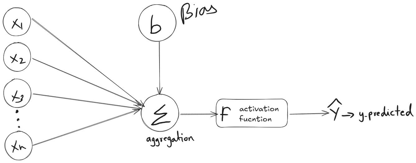
At a glance, an ANN takes inputs, multiplies them by weights (think of this like “how important is this ingredient”), adds some bias (like a pinch of salt), and passes it through an activation function (like deciding whether or not to bake at high heat). This process is repeated across layers until the network spits out a prediction.

One example equation looks like this:

output = activation(weights × input + bias)

At its core, an ANN is just a sequence of linear algebra and functions stacked together. Let’s break it down:

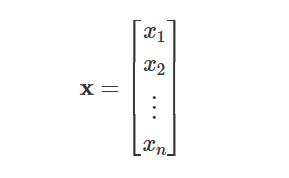
1. Inputs: Represented as a vector

   

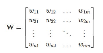
2. Weights: Each connection has a weight, telling the network how important each input is:

   

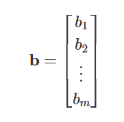
3. Biases: Each neuron also has a bias b that shifts the activation function:

   

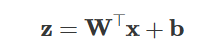
4. Linear combination: Each neuron computes a weighted sum of its inputs plus bias:

   

   Here, z is a vector of “pre-activation” values for the neurons in the layer.

5. Activation function: To introduce non-linearity, each zi passes through a function f, like ReLU, Sigmoid, or Tanh:

   

   We’ll see how non-linear activation functions play a crucial role in helping the network learn complex patterns when we dive into the code later. For now, just know that without these functions, the network wouldn’t be able to capture intricate relationships in the data.

   There’s a lot more to activation functions than we can cover here, so if you’re eager to explore how they really work and why they’re so important, check out this excellent guide by Towards Data Science.

6. Propagation through layers: If the network has multiple hidden layers, this process repeats. For the each layer:

   

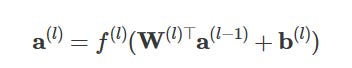
   l is the current layer.

7. Finally, the output layer produces the network’s prediction:

   

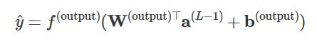
So in short: inputs → weighted sums → add bias → activation → repeat → output.

Think of it like a factory assembly line, each neuron takes in signals, decides how much to pass on using weights and biases, transforms it through an activation, and sends it down the line. Once you frame it like that, those equations stop looking intimidating, they’re just neat, organized matrix multiplications doing their job!

Why PyTorch is awesome

When it comes to building deep learning models, PyTorch stands out as one of the most powerful and user-friendly tools available. It combines ease of use with advanced functionality, which is why so many developers and researchers rely on it. Here’s what makes it such a great choice:

• The interface is intuitive and feels like writing regular Python code.

• It comes with automatic differentiation through autograd, so you don’t have to manually compute gradients.

• It gives you the freedom to experiment, whether you are working on simple models or building more advanced ones.

• It is trusted and widely used by researchers and professionals across different industries.

Let’s build our first ANN with PyTorch

Alright, now that we’ve talked about the math behind neural networks, let’s roll up our sleeves and build two models from scratch! We’ll create a fun problem where data points form circles, definitely not something you can solve with a straight line. First, we’ll see how a model with only linear layers struggles, and then we’ll add a ReLU activation function to show how non-linearity unlocks the power to handle complex patterns.

Step 1 – Import the essentials

Before we jump into the math and data, let’s bring in the tools we need:

import torch
import torch.nn as nn
import torch.optim as optim
import matplotlib.pyplot as plt
import numpy as np

PyTorch helps us build and train models, while Matplotlib and NumPy are here to help us visualize and handle data. It’s like assembling your toolkit before building something awesome!

Step 2 – Set up device-agnostic code

If you have a GPU, great! It’ll speed up training. If not, don’t worry your CPU will handle it.

device = "cuda" if torch.cuda.is_available() else "cpu"
device

You’ll see either "cuda" or "cpu" printed out. Either way, we’re covered!

Step 3 – Making some dummy data

We’re not using real-world datasets for this one. Instead, we’ll create a fun synthetic dataset using circular patterns to clearly see the difference between linear and non-linear models.

from sklearn.datasets import make_circles

# Generate circular data
X, y = make_circles(n_samples=500, noise=0.1, factor=0.5, random_state=42)
X = torch.tensor(X, dtype=torch.float32)
y = torch.tensor(y, dtype=torch.float32).reshape(-1, 1)

# Plot the data
plt.figure(figsize=(6,6))
plt.scatter(X[:, 0], X[:, 1], c=y.squeeze(), cmap='bwr', edgecolor='k')
plt.title("Circular Data Distribution")
plt.xlabel("Feature 1")
plt.ylabel("Feature 2")
plt.show()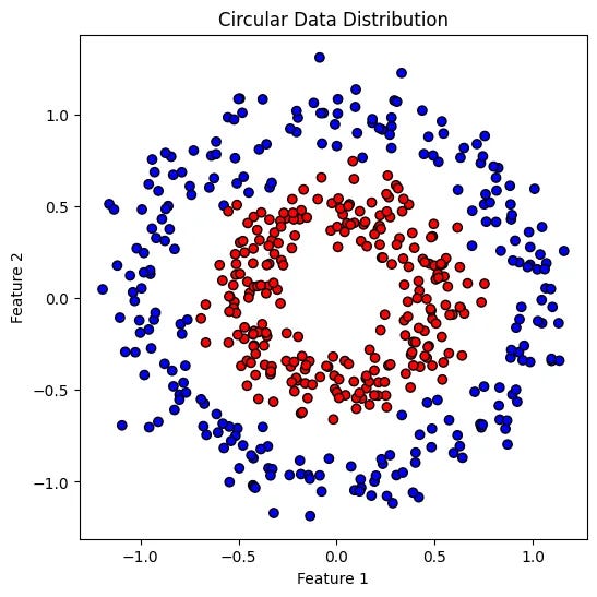

Look at that! One class sits inside the circle while the other surrounds it. A straight line won’t do the job here, and that’s where non-linear activation functions come in!

Step 4 – Splitting the data

We’ll split this dataset into 80% training and 20% testing, just enough to learn and then check how well the model generalizes.

train_size = int(0.8 * len(X))
X_train, X_test = X[:train_size], X[train_size:]
y_train, y_test = y[:train_size], y[train_size:]

Step 5 – Define the Linear Model

This model is like trying to fit a straight edge across curved patterns it’s going to struggle, but it’s an important learning step.

class LinearModel(nn.Module):
    def __init__(self):
        super().__init__()
        self.fc1 = nn.Linear(2, 5)  # 2 input features, hidden units
        self.hidden = nn.Linear(5, 2)  # 5 input features, 2 hidden units
        self.fc2 = nn.Linear(2, 1)  # 2 hidden units, 1 output

    def forward(self,x):
        x = self.fc1(x)
        x = self.hidden(x)
        return torch.sigmoid(self.fc2(x))

It’s simple and neat, but lacks the power to draw curves!

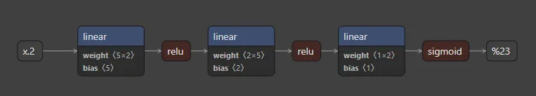
If we visualize this model it will look like this:

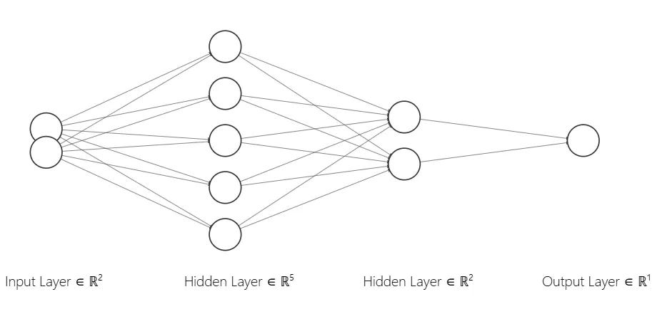
Step 6 – Define the Non-Linear Model

Here’s where things get exciting! We introduce the ReLU activation function, which allows the model to learn complex, curved decision boundaries.

class NonLinearModel(nn.Module):
    def __init__(self):
        super().__init__()
        self.fc1 = nn.Linear(2, 5)   # Input → hidden
        self.hidden = nn.Linear(5, 2)  # Hidden → hidden
        self.fc2 = nn.Linear(2, 1)    # Hidden → output
        self.relu = nn.ReLU()         # Single activation layer reused

    def forward(self, x):
        x = self.fc1(x)
        x = self.relu(x)
        x = self.hidden(x)
        x = self.relu(x)
        x = self.fc2(x)
        return torch.sigmoid(x)

With just one activation function sprinkled in, this model suddenly thinks outside the box, or in this case, the circle!

Step 7 – Initialize the models

Let’s create instances of both models and move them to the correct device.

linear_model = LinearModel().to(device)
nonlinear_model = NonLinearModel().to(device)

Step 8 – Define the training and testing functions

Now, let’s build functions that teach the models how to learn and test their performance on new data.

Training function:

def train(model, X_train, y_train, loss_fn, optimizer, acc):
    X_train, y_train = X_train.to(device), y_train.to(device)
    model.train()
    optimizer.zero_grad()
    y_pred = model(X_train)
    loss = loss_fn(y_pred, y_train)
    preds = (y_pred > 0.5).int()
    accuracy = acc(preds, y_train.int())
    loss.backward()
    optimizer.step()
    return loss.item(), accuracy

Testing function:

def test(model, X_test, y_test, loss_fn, acc):
    X_test, y_test = X_test.to(device), y_test.to(device)
    model.eval()
    with torch.no_grad():
        y_pred = model(X_test)
        loss = loss_fn(y_pred, y_test)
        preds = (y_pred > 0.5).int()
        accuracy = acc(preds, y_test.int())
    return loss.item(), accuracy

Step 9 – Pick the loss function and optimizers

For our binary classification, we’ll use binary cross-entropy loss, and Adam optimizer helps the models learn more smoothly. We could pick any other loss function too like Stochastic GD or Momentum Based GD

criterion = nn.BCELoss()
linear_optimizer = optim.Adam(linear_model.parameters(), lr=0.01)
nonlinear_optimizer = optim.Adam(nonlinear_model.parameters(), lr=0.01)

Step 10 – Training the models

Here’s where the models go through multiple rounds, called epochs of training. Every 50 epochs, we check how well they’re doing.

from torchmetrics.classification import Accuracy

linear_acc = Accuracy(task="binary")
nonlinear_acc = Accuracy(task="binary")

num_epochs = 150

for epoch in range(1, num_epochs + 1):
    linear_train_loss, linear_train_acc = train(linear_model, X_train, y_train, criterion, linear_optimizer, linear_acc)
    linear_acc.reset()

    nonlinear_train_loss, nonlinear_train_acc = train(nonlinear_model, X_train, y_train, criterion, nonlinear_optimizer, nonlinear_acc)
    nonlinear_acc.reset()

    if epoch % 50 == 0:
        linear_test_loss, linear_test_acc = test(linear_model, X_test, y_test, criterion, linear_acc)
        linear_acc.reset()

        nonlinear_test_loss, nonlinear_test_acc = test(nonlinear_model, X_test, y_test, criterion, nonlinear_acc)
        nonlinear_acc.reset()

        print(f"Epoch {epoch}/{num_epochs}")
        print(f"Linear Model -> Train Loss: {linear_train_loss:.4f}, Train Accuracy: {linear_train_acc:.4f}")
        print(f"Linear Model -> Test Loss: {linear_test_loss:.4f}, Test Accuracy: {linear_test_acc:.4f}")
        print(f"Nonlinear Model -> Train Loss: {nonlinear_train_loss:.4f}, Train Accuracy: {nonlinear_train_acc:.4f}")
        print(f"Nonlinear Model -> Test Loss: {nonlinear_test_loss:.4f}, Test Accuracy: {nonlinear_test_acc:.4f}")
        print("-------------------------------")

This is where you’ll see the models learn or struggle in real time!

Output:

Epoch 50/150
Linear Model -> Train Loss: 0.6927, Train Accuracy: 0.4925
Linear Model -> Test Loss: 0.6967, Test Accuracy: 0.4200
Nonlinear Model -> Train Loss: 0.6175, Train Accuracy: 0.6100
Nonlinear Model -> Test Loss: 0.6415, Test Accuracy: 0.5800
-------------------------------
Epoch 100/150
Linear Model -> Train Loss: 0.6927, Train Accuracy: 0.4400
Linear Model -> Test Loss: 0.6971, Test Accuracy: 0.3900
Nonlinear Model -> Train Loss: 0.4151, Train Accuracy: 0.8750
Nonlinear Model -> Test Loss: 0.4450, Test Accuracy: 0.8200
-------------------------------
Epoch 150/150
Linear Model -> Train Loss: 0.6927, Train Accuracy: 0.4350
Linear Model -> Test Loss: 0.6971, Test Accuracy: 0.3800
Nonlinear Model -> Train Loss: 0.1636, Train Accuracy: 0.9825
Nonlinear Model -> Test Loss: 0.2039, Test Accuracy: 0.9400
-------------------------------

You won’t believe how huge the difference is! The linear model barely improves it’s stuck guessing around 40–50% accuracy, like flipping a coin. Meanwhile, the nonlinear model crushes it, achieving over 98% training accuracy and 94% on test data, proving that a little non-linearity goes a long way in solving complex problems!

Step 11 – Evaluating the models with confusion matrices

Let’s check how well the models are doing by comparing their predictions to the actual answers.

from torchmetrics.classification import ConfusionMatrix
import seaborn as sns

confmat = ConfusionMatrix(task="binary")

linear_model.eval()
nonlinear_model.eval()
with torch.inference_mode():
    linear_preds = linear_model(X_test)
    nonlinear_preds = nonlinear_model(X_test)

linear_preds = (linear_preds > 0.5).int()
nonlinear_preds = (nonlinear_preds > 0.5).int()
targets = y_test.int()

linear_cm = confmat(linear_preds, targets)
nonlinear_cm = confmat(nonlinear_preds, targets)

def plot_confusion_matrix(cm, title):
    plt.figure(figsize=(5,4))
    sns.heatmap(cm.cpu().numpy(), annot=True, fmt='d', cmap='Blues')
    plt.xlabel("Predicted")
    plt.ylabel("Actual")
    plt.title(title)
    plt.show()

plot_confusion_matrix(linear_cm, "Confusion Matrix - Linear Model")
plot_confusion_matrix(nonlinear_cm, "Confusion Matrix - Nonlinear Model")

The confusion matrix is like a scoreboard, it shows how many times the models got it right or wrong!

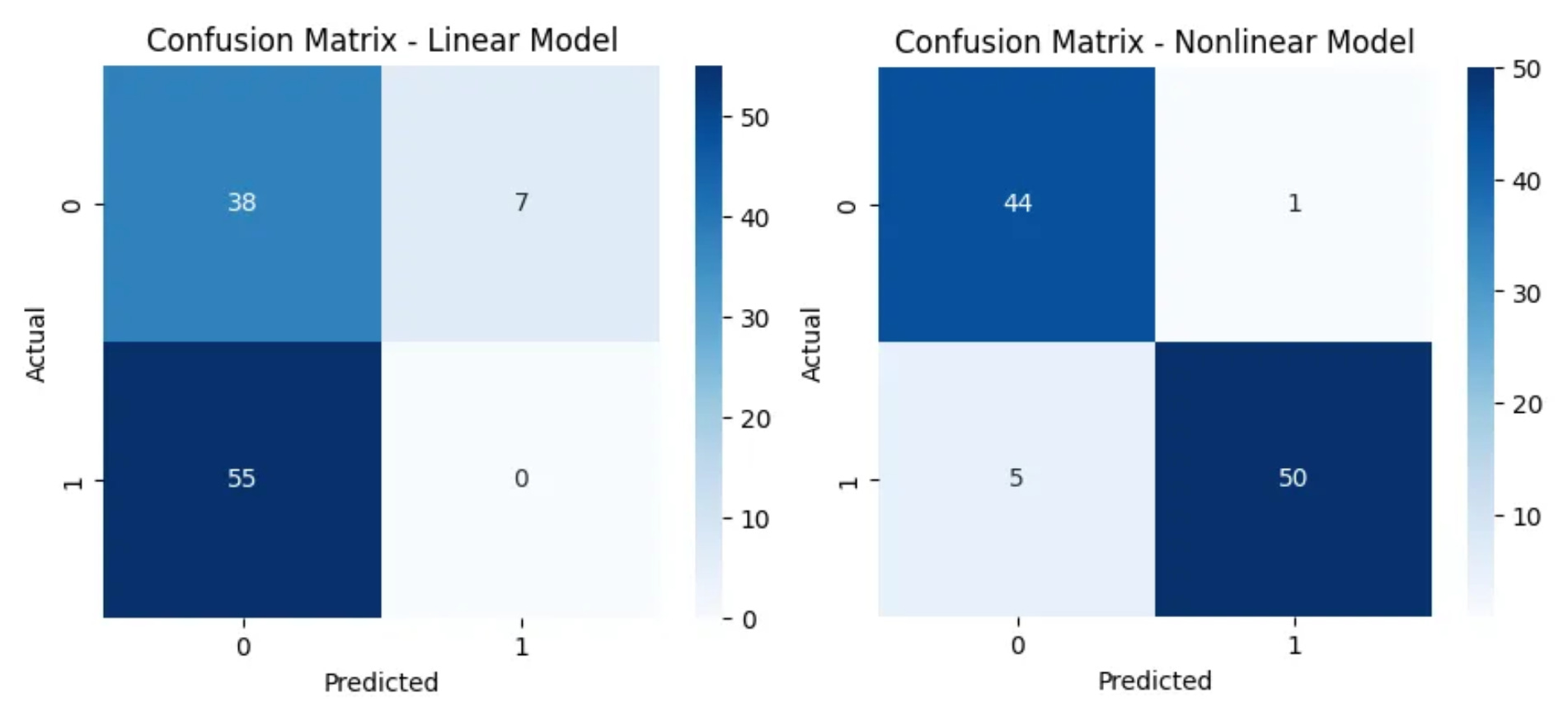
Look at how much clearer the nonlinear model’s predictions are. It’s nailed it with 44 true negatives and 50 true positives, barely mixing things up with just a couple of mistakes. Meanwhile, the linear model is really struggling, it’s misclassifying way more, especially with 55 false negatives. It almost always guesses class 0, which is a hit or a miss, proving that without non-linearity, it just can’t wrap its head around the complexity of the data!

Step 12 – Visualize decision boundaries

Finally, let’s draw how the models are classifying the space. It’s like tracing their thought process!

def plot_decision_boundary(model, title):
    model.eval()
    x_min, x_max = X[:, 0].min() - 0.5, X[:, 0].max() + 0.5
    y_min, y_max = X[:, 1].min() - 0.5, X[:, 1].max() + 0.5
    xx, yy = np.meshgrid(np.linspace(x_min, x_max, 200),
                         np.linspace(y_min, y_max, 200))
    grid = torch.tensor(np.c_[xx.ravel(), yy.ravel()], dtype=torch.float32).to(device)
    with torch.inference_mode():
        preds = model(grid).reshape(xx.shape).cpu().numpy()
    plt.contourf(xx, yy, preds, levels=[0, 0.5, 1], cmap='bwr', alpha=0.3)
    plt.scatter(X[:, 0], X[:, 1], c=y.squeeze(), cmap='bwr', edgecolor='k')
    plt.title(title)
    plt.xlabel("Feature 1")
    plt.ylabel("Feature 2")
    plt.show()

plot_decision_boundary(linear_model, "Decision Boundary: Linear Model")
plot_decision_boundary(nonlinear_model, "Decision Boundary: Non-Linear Model with ReLU")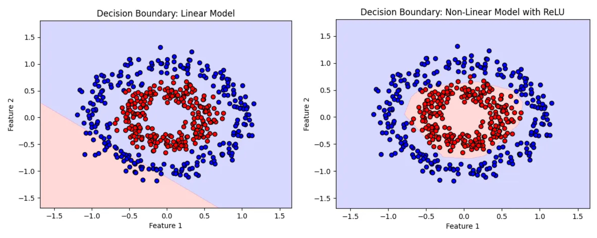

Check out these decision boundaries! The nonlinear model with ReLU has carved out a beautiful, curved boundary that perfectly wraps around the circular patterns in the data. On the other hand, the linear model draws a straight line, missing most of the structure and barely separating the classes, it’s like trying to fit a round peg into a square hole. This really shows how powerful non-linearity is when it comes to understanding complex patterns.

Its time to wrap up the code implementation, if you enjoyed this walkthrough try tweaking the number of hidden neurons or playing with learning rates and see how the results change. You can explore the full implementation of both the linear and non-linear models, including the circular dataset, training code, and decision boundary visualizations, in the notebook here.

Key Takeaways:

• Linear layers alone can only create straight decision boundaries.

• Non-linear activation functions like ReLU allow the network to approximate complex, non-linear patterns in data.

• Even a single hidden layer with non-linear activation can drastically improve a model’s capability on non-linear datasets.

Common mistakes you’ll probably make (and it’s okay!)

• Shape errors – “Expected input to have shape…” → check dimensions carefully.

• Forgetting .backward() or optimizer.step() → training won't happen!

• Wrong learning rate – too small and it crawls; too large and it overshoots the minima, causing oscillation.

• Device mismatch – tensors and model must be on the same device (cpu vs cuda); otherwise you'll get errors like Expected all tensors to be on the same device.

Always write device agnostic code, print shapes and loss after each step, it’s your debugging lifeline!

Where to go next?

Once you've grasped the fundamentals of neural networks, you can learn about more specialized architectures. Here's a what you could do next:

• Convolutional Neural Networks (CNNs): Essential for tasks like image classification and object detection. We'll delve into CNNs next Monday, 22 September 2025, where we'll explore how these networks analyze and interpret visual data.

• Recurrent Neural Networks (RNNs): Ideal for processing sequential data such as time series or text. Our blog post, "Giving Words Meaning with RNNs", provides an overview of RNNs and their applications.

• Long Short-Term Memory (LSTM) Networks: A specialized type of RNN designed to capture long-term dependencies. For a comprehensive understanding, check out our blog post, "Fixing a Broken Memory with LSTMs", where we discuss how LSTMs address the limitations of traditional RNNs.

• Transformers: The backbone of modern language models like GPT, BERT, and T5. We'll explore transformers in detail in upcoming blog post, focusing on their architecture and applications in natural language processing.

Each of these architectures builds upon the concepts we've covered, offering powerful tools for tackling a wide range of problems in machine learning and artificial intelligence.

Final thoughts

Remember, deep learning isn’t just about memorizing formulas or writing code, it’s about developing intuition, experimenting thoughtfully, and understanding how models learn. Explore different architectures, adjust the number of neurons, try alternative activation functions, and analyze decision boundaries. Each experiment provides valuable insight into how neural networks process information and make predictions.

The techniques you’ve practiced today are the foundation for addressing real-world problems, from forecasting trends to analyzing medical images. Approach your learning methodically, test your ideas, and reflect on the outcomes, this is how progress in AI is made.

Resources

To help you continue your journey in neural networks and PyTorch, here are some hand-picked resources:

1. Official PyTorch Documentation

   Comprehensive guides, tutorials, and API references straight from the creators.

2. Neural Networks and Deep Learning by Michael Nielsen –

   A free, beginner-friendly book that explains the math and intuition behind neural networks.

3. 3Blue1Brown: “But what is a neural network?”

   A visual and intuitive introduction to neural networks with stunning animations that make complex concepts easy to grasp.